Encoding Symbolic Expressions as Efficient Solver Queries
This post was originally published on the blog of Dependable Systems Lab at EPFL.
Constraint solving constitutes a major bottleneck in symbolic execution. It is therefore important to maximize solver performance, which in turn can improve path throughput, code coverage, and the number of bugs discovered. In this post, we show that the encoding of symbolic expressions as solver queries significantly impacts the solver performance. By exploring a few points in the design space of query encodings, we discovered performance differences spanning over two orders of magnitude. On a Chef symbolic execution workload, the Z3 constraint solver achieved the best performance when running in a portfolio of incremental and non-incremental configurations, by encoding memory accesses as operations over the array theory and using assertions to initialize constant arrays.
The symbolic execution literature mainly covers two factors that affect the performance of the constraint solver: (1) the choice of the solver itself and (2) the complexity of the symbolic expressions reaching the solver. For the former, efforts such as metaSMT provide a uniform interface for expressing queries in a theory and targeting multiple solvers. Moreover, previous research demonstrated the benefits of running different solvers in parallel, as a portfolio. The latter factor was also studied and techniques such as expression simplification and caching showed significant performance improvements.
However, there is a third factor that significantly affects the solver performance and that has been less studied: the conversion from the engine-specific symbolic expressions to solver queries. Symbolic expressions are constructs that encompass program operations, such as memory accesses. In some sense, they are static representations of the program’s symbolic execution state, whereas solver queries have a lower-level representation and consist of statements that manipulate the current solver state.
This post shows that the gap between symbolic expressions and solver queries can be bridged in several ways, each with a different performance profile. We explore two dimensions of the solver query encoding design space: the encoding of memory operations and the leverage of solver incrementality mechanisms.
We implemented several points in the design space using the Z3 constraint solver, with a 110× performance difference between the fastest and slowest configuration. We discovered that a portfolio of incremental and non-incremental solver configurations achieve the best performance on a Chef symbolic execution workload with state merging enabled, 2.25× faster than the purely non-incremental configuration, which was the fasest single-solver configuration.
This post sums up our recent experience of finding the best interface to a constraint solver. Although the results are Z3 specific, they highlight the optimization opportunitites in the solver/engine interface. This post aims to raise awareness among symbolic execution engine authors and invites for deeper research on the topic.
In the rest of this post, we give a brief overview of constraint solvers, present the design space of encoding memory operations and of leveraging solver incrementality, present our experimental results using the Z3 solver, then conclude with a discussion on limitations and future work.
1. Constraint Solving Primer
Modern constraint solvers are programs specialized in answering the following type of queries: “Is the boolean expression \(e\), expressed in theory \(T\), satisfiable?” Here, the theory \(T\) is the “language” of the expression \(e\). For example, the bitvector theory (more formally, the quantifier-free theory of bitvectors, or QF_BV) defines the arithmetic and logic operations over binary integers. Popular solvers used in symbolic execution include STP, Z3, Boolector, CVC4, and MathSAT.
As the satisfiability problem is generally NP-hard, solvers resort to various strategies tailored to the specifics of each theory. However, the solver performance is unpredictable and may vary drastically across workloads.
Most symbolic execution engines use the theory of bitvectors and arrays (QF_ABV), as it allows an accurate and concise representation of program operations. QF_ABV extends QF_BV with read and write operations on array variables, which are used to represent program memory. For example, the KLEE symbolic execution engine uses a solver array variable for each symbolic memory block malloc()-ed by the program, while the S2E VM-level symbolic execution engine uses an array variable for each symbolic page of physical memory in the VM.
The symbolic execution engine constructs the solver query \(e\) through a command interface that allows the engine to declare assertions and invoke satisfiability checks. For example, the command sequence \(\mathrm{assert}(p);\;\mathrm{assert}(q);\;\mathrm{checksat}()\) results in the solver computing the satisfiability of \(p \wedge q\).
2. Encoding Memory Operations
Each path condition constructed by the symbolic execution engine must be converted into a solver query, in order to decide its feasibility. Most operations in symbolic expressions, such as arithmetic and logic, have a straightforward one-to-one mapping in the QF_ABV theory. However, memory operations do not have a direct, obvious mapping, so the engine must encode them as simpler QF_ABV solver expressions. In this section, we present several design choices of encoding memory operations.
Memory operations consist of reading and writing bytes from memory locations. There are two common ways to represent these operations: by using read/write expressions over array variables, or by explicitly instantiating the array theory as nested if-then-else expressions.
Array Expressions. With array expressions, there is a one-to-one mapping between the read and write memory operations and the correspoding array theory operations. There is one caveat, though: the array theory works with immutable arrays, such that writing value \(v\) to array \(A\) at index \(i\) (i.e., \(\mathrm{write}(A, i, v)\)) produces a new array with the updated value. Hence, \(\mathrm{read}(A, i)\) operations are applied on expressions consisting of nested \(\mathrm{write}\) operations that construct the contents of the array read from.
The nested writes representation may be expensive for initializing arrays with constant values, as the nesting depth equals the size of the array. As a result, some solvers, such as Z3, deal more efficiently with arrays initialized through assertions, i.e. \(\mathrm{assert}(\mathrm{read}(A, i)) = v)\).
If-Then-Else Expressions. An alternative to using arrays is to explicitly create if-then-else (ITE) expressions that instantiate the array axiom \(\mathrm{read}(\mathrm{write}(A, i, v), j) = v \;\mathbf{if}\; i == j \;\mathbf{else}\; \mathrm{read}(A, j)\). This method is preferred in particular cases where the array size is small or its usage limited to certain patterns. For example, the Mayhem symbolic execution engine uses the ITE form to encode symbolic reads, while restricting all writes to concrete indices.
3. Solver Incrementality
Many solver interfaces offer an incremental construction of solver queries. Instead of rebuilding the assertions from scratch for each satisfiability check, the solver provides a stateful session (also called context) in which variables and assertions are defined and removed as needed. For example, the command sequence \(\mathrm{assert}(p);\;\mathrm{checksat}();\;\mathrm{assert}(q);\;\mathrm{checksat}()\) reuses in the second query the assertion of \(p\) from the first query. Beside the conciseness benefits, incremental queries may also be solved faster, as the solver can reuse knowledge gained from previous queries.
Mechanisms
Incrementality is most useful in symbolic execution when assertions can be both enabled and retracted, as needed. To this end, most solvers provide two mechanisms: context stacks and assumptions.
Context Stacks. In one form of incrementality, the solver context, which includes variables, assertions, and the knowledge gained from previous checks, can recursively be saved and restored with \(\mathrm{push}()\) and \(\mathrm{pop}()\) operations.
For example, if a symbolic execution engine checks the feasibility of path condition \(c_1 \wedge c_2\), followed by \(c_1 \wedge c_3\), the solver command sequence that uses context stacks is \(\mathrm{assert}(c_1);\;\mathrm{push}();\;\mathrm{assert}(c_2);\;\mathrm{checksat}()\), followed by \(\mathrm{pop}();\;\mathrm{assert}(c_3);\;\mathrm{checksat}()\).
Assumptions. Assumptions can be used to enable and disable assertions for each \(\mathrm{checksat}\) request. Unlike context stacks, any assertion can be disabled, not only the most recent. Solvers have different ways of providing assumptions.
For example, in Z3, assumptions are guarded assertions, i.e., assertions that are conditioned by a boolean variable. By using Z3 assumptions, our previous example can be rewritten as \(\mathrm{assert}(\mathbf{b_1} \rightarrow c_1);\;\mathrm{assert}(\mathbf{b_2} \rightarrow c_2);\;\mathrm{checksat}(\mathbf{b_1} \wedge \mathbf{b_2})\), followed by \(\mathrm{assert}(\mathbf{b_3} \rightarrow c_3);\;\mathrm{checksat}(\mathbf{b_1} \wedge \mathbf{b_3})\).
Resetting the Solver State
Maintaining the assertions and knowledge from previous queries (we call it query history) is ostensibly better than solving a new query from scratch. However, accumulating query history carries an overhead. Each new assertion is propagated in a database of existing assertions and lemmas, which can take considerable time when the database is large. Therefore, incrementality is only worthwhile if the query history includes an insight that helps the solver reach a conclusion faster and offset the overhead of maintaining the history.
Consequently, an incremental solver that continuously accumulates query history would eventually run out of memory or slow down to the point it becomes unusable. Hence, the query history should be capped to a maximum size.
A simple approach to limit the query history overhead is to periodically reset the solver state. For example, in the case of assumption-based incrementality, the solver can be reset once the number of assumptions reaches a fixed threshold value. In general, an adaptive threshold could also be employed. In either case, choosing the reset points is a heuristic matter. On the one hand, having too little history may cause the solver to redo work. A non-incremental solver is a special case of zero history. On the other hand, too much history would slow the solver during queries that do not use insights from the history.
The Expression Cache
Finally, there is one caveat when interfacing a symbolic execution engine with an incremental solver: the expression cache. To avoid redoing work, a symbolic execution engine typically caches the symbolic expressions converted to a solver representation, so entire sub-expressions can be simply reused when they are encountered multiple times.
When the solver is incremental, the cache needs to be kept in sync with the solver state. For example, in the case of context stack incrementality, whenever a context is popped, the variables and expressions created for the popped context should be removed from the cache. A trivial approach is to simply reset the cache after each popped context, but this results in redundant work. A more refined approach is to represent the cache as a stack of snapshots that are pushed and popped in sync with the solver. An immutable map is a data structure for the cache that can be efficiently snapshotted.
4. Experimental Results
In this section, we evaluate the performance of constraint solving under a combination of incrementality configurations and memory operation encodings.
Setup
We collected 33,009 path conditions during a run of the Chef symbolic execution platform for interpreted languages. Chef supports interpreted languages by running the interpreter binary inside a VM-level symbolic execution engine (S2E).
For our experiment, Chef was configured to execute a symbolic test for the argparse standard Python package, by using the vanilla Python 2.7.3 interpreter.
During execution, we enabled state merging, which resulted in path conditions containing disjunctive expressions, notoriously difficult for a constraint solver.
We used the Z3 solver, which provided competitive performance and allowed us to implement the different configurations of incrementality and memory encoding. We interfaced with the solver using its native C++ interface, by extending the KLEE-based solver subsystem used in S2E.
We encoded Z3 queries under four configurations of incrementality and memory encoding, presented in the table below:
| Incrementality | Memory Encoding | Queries Replayed | Total Time (or Slow-down) |
|---|---|---|---|
| None | Arrays (Asserts) | 33,009 | 2h 29m 40s |
| Arrays (Writes) | 4,240 | 49.76× | |
| If-Then-Else | 10,904 | 11.18× | |
| Assumptions | Arrays (Asserts) | 33,009 | 2.33× |
For each Z3 configuration, we constructed the solver queries in the order they were recorded during symbolic execution. For the configurations incurring a significant slowdown, we stopped the process before all queries were solved (the warning signs in the table). We compared configurations based on the commonly solved queries.
For the array-based memory encoding, we used both nested writes and assertions to initialize constant arrays (the first two rows in the table).
For the assumption-based incrementality, we used a fixed reset threshold of 50 assumptions, as we empirically noticed that it gives a good performance trade-off for our workload.
Result Summary
We present a summary of the results, followed by a more detailed analysis. To enhance readibility, we present speed-up values in green and slow-down values in red.
-
Among the four configurations, the Z3 assert-based non-incremental configuration performs the best overall (first row, in green, in the table above). This configuration is also 1.92× faster than STP, the standard solver used in KLEE-based symbolic execution engines.
-
The incremental configuration incurs a 2.33× slowdown overall, compared to the non-incremental configuration.
-
However, a portfolio consisting of both incremental and non-incremental configuration produces up to 2.25× speed-up over the non-incremental one! A portfolio consists of solver configurations running in parallel for each query, whose answer is returned by the fastest solver for the query. The result is a theoretical upper bound, because it does not account for the implementation overhead of a real portfolio system.
-
Our experiments confirm that Z3 does not handle well constant arrays initialized as nested writes. The slowdown recorded for the first 4,240 queries in the workload is almost 50×.
-
The If-Then-Else representation is not appropriate for arbitrary symbolic memory writes and reads, especially in the presence of state merging. The slowdown recorded for the first 10,904 queries is over 11×.
-
Z3’s performance is sensitive to its configuration and gives best results when it is explicitly configured with the QF_ABV theory.
Comparing Assertions with Nested Writes in Array Initialization
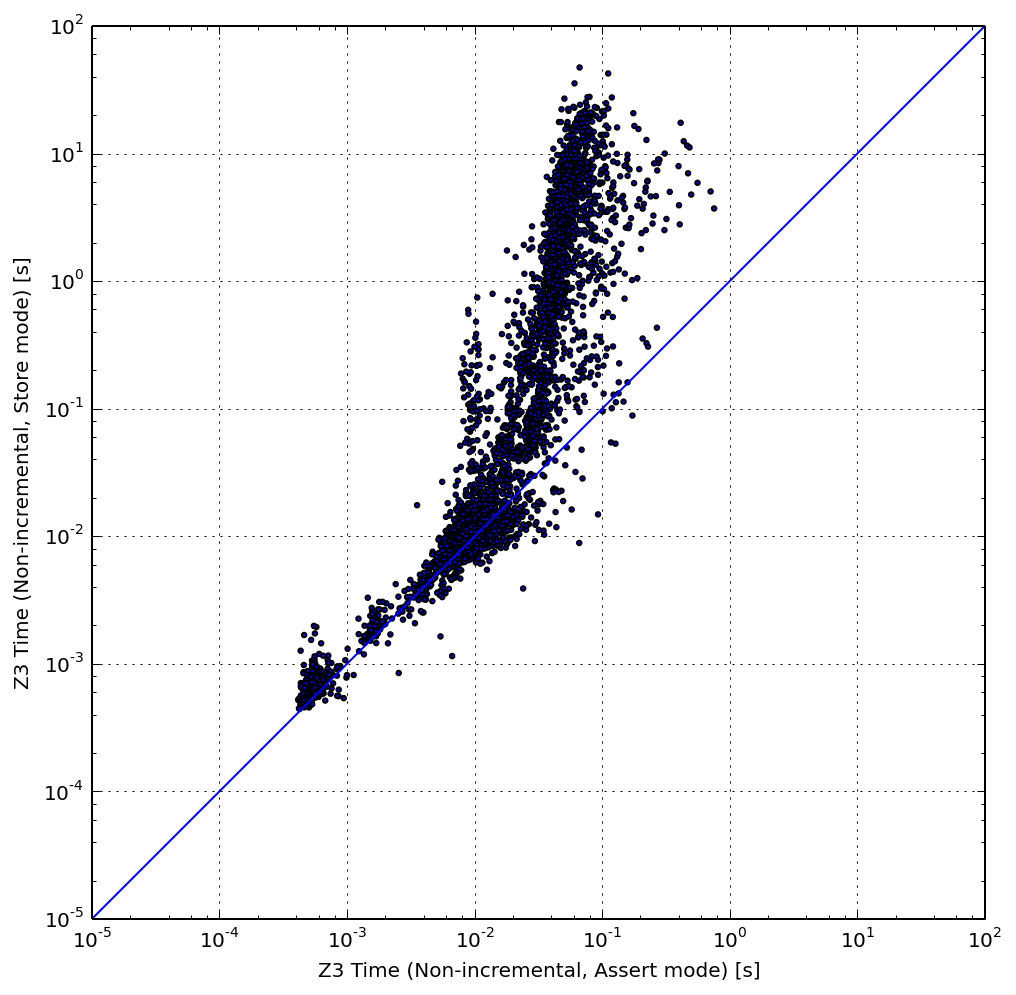
The scatter plot above shows the per-query performance of the non-incremental array-based configuration with assertions used to initialize arrays (X axis), compared to a similar configuration with nested writes used to initialize arrays (Y axis). Each point in the graph represents a query. The queries above the diagonal are solved faster in the assert mode.
The figure shows that most queries are faster in the assertion configuration. Moreover, the gap widens significantly as queries become more expensive.
If-Then-Else Encoding Performance
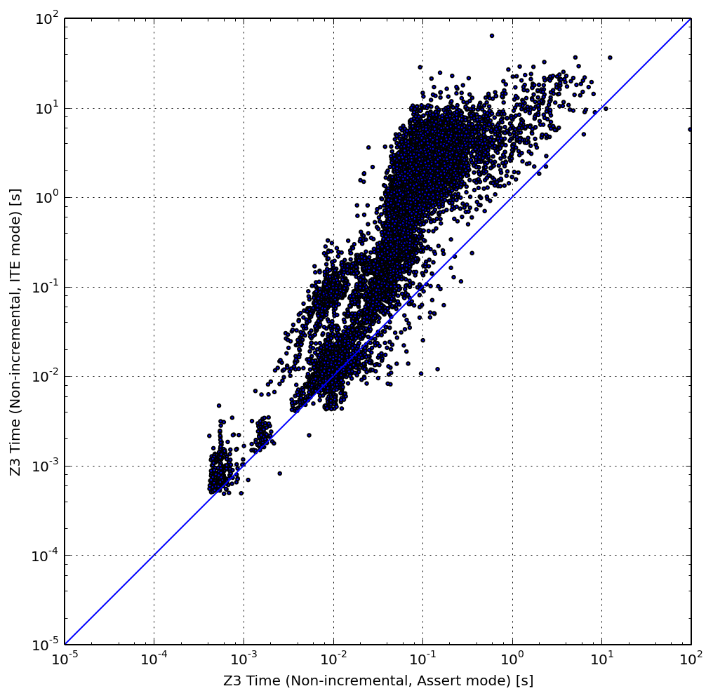
Above is a similar graph that compares the array with assertions configuration (X axis) to the ITE configuration (Y axis). Similarly, the cluster of points veers above the diagonal, showing that the ITE representation is inefficient in our workload.
It is worth mentioning that the ITE representation is still useful when the combinatorial explosion of matching all reads with all writes in the nested ITE chains can be reduced. For example, it is successfully being used in the Mayhem symbolic execution engine, where the memory writes are restricted to concrete addresses. For that case, the general-purpose array theory built into the solver may be less efficient.
Incrementality Performance
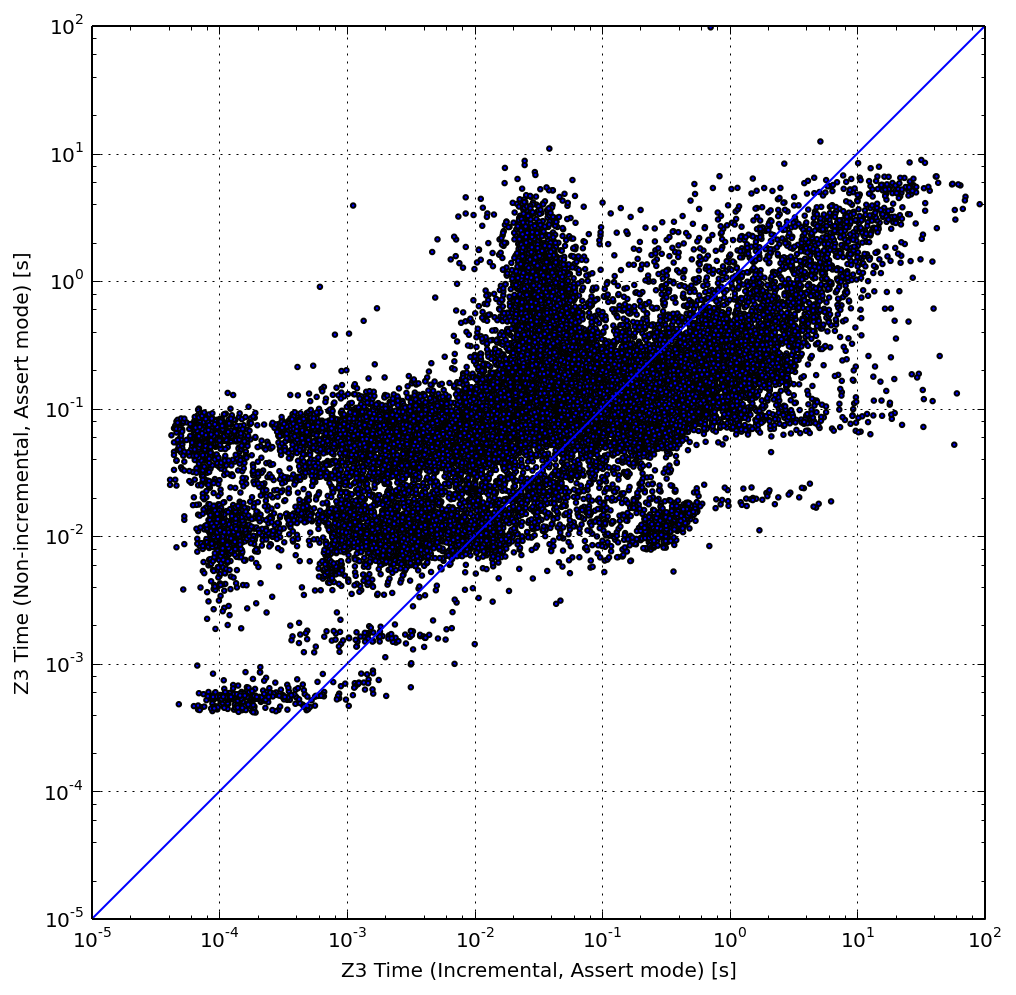
We evaluated the performance of Z3’s incrementality support by comparing the best performing non-incremental configuration (the array memory encoding, with assertions, on the Y axis) to its incremental assumption-based variant (X axis). The graph above shows the comparison for each query in the workload.
Overall, most query points tend to be above the diagonal, where the incremental Z3 is more efficient. However, the graph shows that the more expensive queries (on the right) tend to slow down in incremental mode (they are below the diagonal). Since these queries dominate the total execution time, they slow down the overall performance of the incremental solver by 2.33×.
Recall that the cost of incrementality is worthwhile only if the query history stored in the solver state includes an insight that helps the solver to reach a conclusion faster. The results show that this is the case only for a fraction of the queries.
Since each of the solver configurations has a query subset where it performs significantly better, a solver portfolio would improve the system performance. The idea is to run both solver configurations in parallel for each query, and proceed when the fastest solver for the query gives an answer.
From our experiments, a portfolio of the incremental and non-incremental configurations would achieve a speed-up of 2.25× over the non-incremental mode, without considering any implementation overhead. This speed-up is also useful from a resource utilization standpoint, as the per-CPU scalability is super-linear. If this was not the case, we may not have been using efficiently the CPU resources. For example, instead of using 2 CPUs for the solver portfolio, we could have used them to parallelize symbolic execution itself.
In conclusion, this result shows that incrementality is useful when used in conjunction with a non-incremental configuration.
Other Z3-Specific Observations
During our experimentation with Z3, we took note of several interesting behaviors:
-
Z3’s performance is highly sensitive to its theory configuration. In its default configuration, Z3 appears to use a general-purpose solving strategy, which is significantly slower than the strategy used when explicitly configuring the solver with the QF_ABV theory.
-
Similarly, the QF_BV (pure bitvector) theory was less efficient than QF_ABV for the ITE-encoded queries. We found this result surprising, as those queries did not contain any array variables, so QF_BV should have performed at least as good as QF_ABV.
-
When running in incremental mode (context stacks or assumptions), Z3 exhibits some extra overhead, irrespective of the query history. This appears to be caused by Z3 using a different solving strategy as soon as an incremental operation is performed. In our experiments, when given a single entire query to solve with no query history, incremental Z3 is about 20% slower than non-incremental Z3, in the arrays-with-assertions configuration.
5. Limitations and Future Work
Our experiments indicate that the way path conditions are encoded as solver queries significantly influences the solver performance. The total solver times we collected with four Z3 solver configurations vary across two orders of magnitude.
That being said, this study has limitations. There are also more questions that are being left unanswered.
Generality of Results. The major limitation of this study is that only a single solver was considered (Z3), on a single symbolic execution workload (the argparse Python package), from a single symbolic execution engine (Chef). This is certainly not enough to draw any general conclusions over the results. An extended version of this work should include a wider class of solvers and symbolic execution workloads.
Solver Configuration Prediction. As each solver configuration performs best only on a subset of queries, a way to speed up constraint solving is to determine a priori which solver configuration to use for each query. The portfolio approach deals with it by trying out all configurations in parallel, but this uses up extra CPU resources. An alternative is to learn which query features predict best the solver configuration and apply a machine learning algorithm that selects a configuration based on query features. Such features could be the query AST size, the number of nested array operations, the number of ITE nodes, etc. It would be particularly interesting to see how some of the modern learning techniques, like deep learning, work on solver queries.
Multi-Session Solvers. The performance of an incremental solver is heavily influenced by the query ordering, which in turn is determined by the search strategy of the symbolic execution engine. For example, incrementality tends to be more efficient if the engine completes execution paths one by one than if it constantly alternates between paths. In the latter case, the solver would need to maintain the query history of both paths, which adds overhead. Rather than constraining the search strategy, the symbolic execution engine could maintain independent solver sessions for each execution path. When a path forks during symbolic execution, its solver session would also be duplicated. Each solver session would then achieve ideal incrementality, where each query is a superset of the previous.
Acknowledgements. I thank Martin Weber for his help with collecting the path conditions and Baris Kasikci for insightful discussions.